Exploring Properties of Addition and Multiplication with Integers

This is the third in the series of explorations of the properties of addition and multiplication with different number sets. After considering the set of (i) Whole numbers and (ii) Non-negative rational numbers¹, in this article we will deal with the integers. This is a good time to reflect on the series − its need and aspiration.

Why are we doing this series?

The seed idea for this series came from the Handbook on Multiplication in At Right Angles, March 2013 issue where Padmapriya Shirali mentioned how the commutative, associative and distributive properties of multiplication can be verified visually for the set of whole numbers.

The more popular approach to justifying them involves taking any two (or three) whole numbers, computing both LHS and RHS of the number fact we want to establish (e.g. 3 × 7 = 7 × 3, (5 × 4) × 9 = 5 × (4 × 9), etc.) and checking that they are the same. This is an inductive process.

However, Padmapriya’s approach can be generalized for any combination of two or three whole numbers regardless of how large they may be. If we agree that any whole number can be represented by that many counters, then her processes would work for any combination of whole numbers. It may be difficult or impossible to arrange counters for big enough numbers, but it can surely be visualised. Her processes free one from computing on a case-by-case basis, i.e., an inductive process and encourages one towards a deductive process. The generalizability is at the heart of the deductive aspect of these visual approaches.

So, we wanted to explore this approach for commutative and associative properties of addition with whole numbers. In addition, we wanted to explore these properties for addition and multiplication for other number sets viz. (i) fractions (including whole numbers) i.e. non-negative rational numbers, (ii) integers, (iii) rational numbers and (iv) real numbers − in short, all the number sets children encounter up to the secondary level. We ran into certain issues with some of these number sets and will discuss them at the end of the series. At the same time, we could come up with ‘almost proof’ for some of the cases − ‘almost proof’ in the sense that we went from some established results through a series of logical deductive steps to the result we wanted to establish. The ‘almost’ refers to the visual approach or pattern approach taken in establishing some of the results. In the remaining cases, we could come up with purely visual approaches similar to Padmapriya’s.

It is important to note that visualisation of specific cases is different from visuals that can be extended to the general case under consideration. The latter is essentially Proof Without Words (PWW). However, many consider PWWs different from deductive proof.

What have we done so far?

We have published the following so far in one article and a poster in the July 2018 and March 2019 issues respectively:

• Commutative and associative properties of addition for whole numbers through visualisation and an activity respectively − both generalisable for any combination of whole numbers.
• All five properties for addition and multiplication for fractions − all through visualisations with generalisation for any combination of fractions (and whole numbers).

Where do we go from here?

We want to complete the series with three more articles:

1. All five properties of the two operations (i.e., addition and multiplication) with integers – we have used coloured counters (mentioned and used extensively in the Handbook on Integers in At Right Angles, November 2016 issue) for commutative and associative properties of addition and for distributive property of multiplication. We could provide deductive reasoning for the remaining two properties of multiplication based on the three multiplication facts established through patterns (details later).
2. An alternative visual model of multiplication based on scaling with the use of number lines. This is needed to establish similar multiplication facts for non-discrete and negative numbers viz. rational and real.
3. All five properties of the two operations with rational and real numbers. This will involve generalization to coloured lengths and coloured areas from the counters. However, coloured volume will not be required since deductive arguments, similar to integers, will work.

Now let us dive into the set of integers. This set doesn’t have the advantage of non-negativity. But it is a discrete set.

Children usually meet integers in their upper primary when they are more capable of understanding patterns and logical arguments. However, even though the terms commutativity, associativity and distributivity may appear, they are not usually justified in any way other than case by case computation. Most textbooks conveniently assume the commutativity of multiplication for integers especially while defining positive times negative and negative times positive. We feel that the definition of multiplication should be separated and that it should precede the properties.

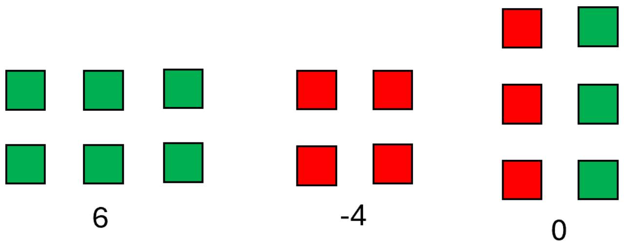
We have used green and red counters as positive and negative units respectively following the Integer Handbook. In this case, square counters have an edge over the round ones. We explain the advantage of squares later. So, six is represented by six green counters, negative four (−4) by four red counters and zero by the absence of any or by equal number of red and green counters (Figure 1).

Addition is modelled in a manner similar to the whole number case. Each integer is represented by that many counters of the right colour. These sets of counters are arranged left to right according to the given addition expression. The combined set of all counters represents the sum. There is an extra step of removing zero pairs. However, this step is not crucial for our purpose.

Commutative Property of Addition

The basic idea behind commutative property is looking at a sum from two vantage points as in the case of whole numbers and fractions.

When it comes to integers, there are four possibilities:

1. Positive + positive
2. Positive + negative (and ∴ negative + positive)

• Sum > 0
• Sum < 0

3. Negative + negative

1 is identical to whole numbers. We have shown an example in Figures 2 and 3 for 2b. The reader can (and should) explore 2a and 3 in similar manner.

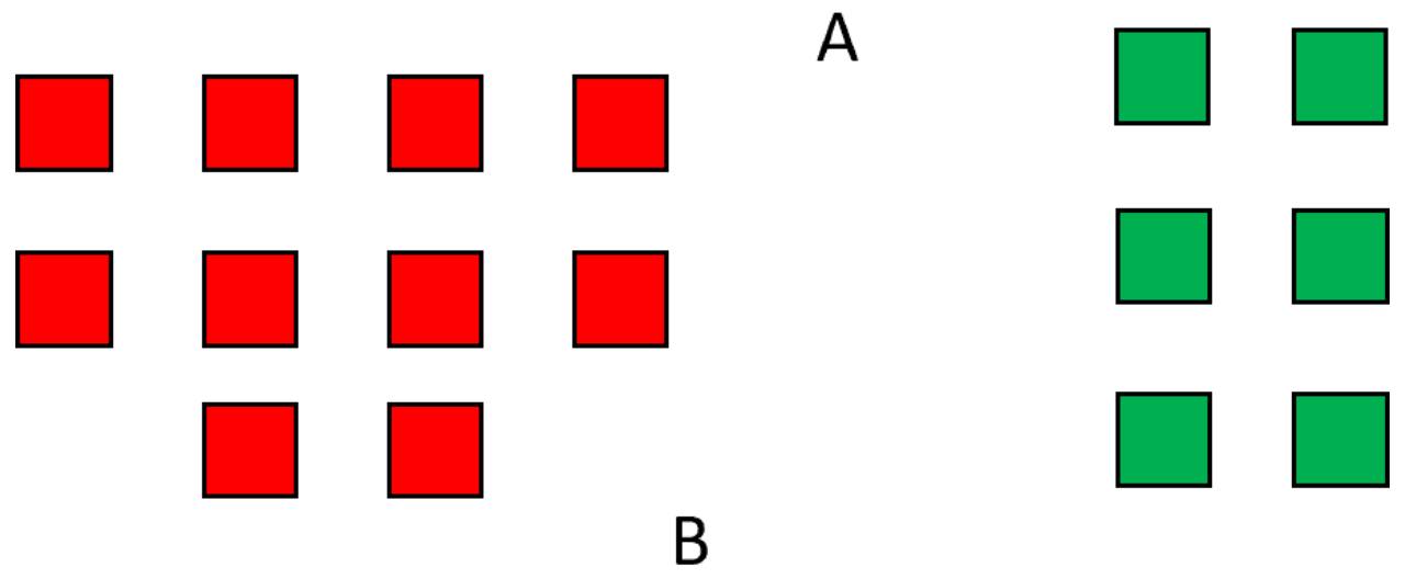
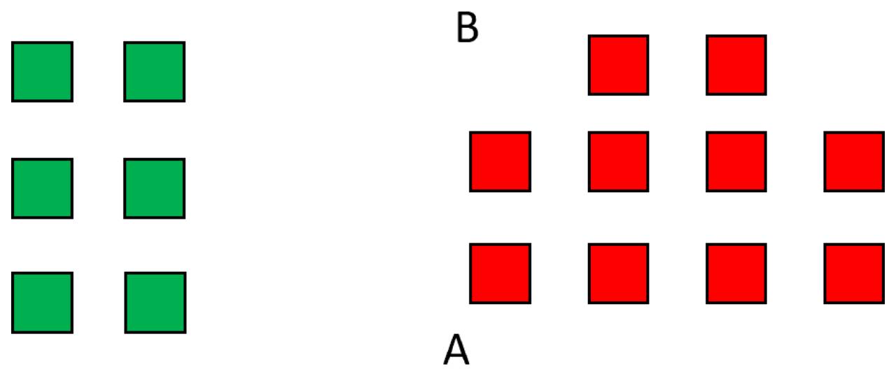
Figure 2 is from B’s perspective and it shows (‒10) + 6 while Figure 3 shows the same sum from A’s view point and it is 6 + (‒10). Since only the perspective changes, the sums remain unchanged, i.e., (‒10) + 6 = 6 + (‒10). Note that this holds for any two integers no matter how far from zero, i.e., how ever many counters may be needed to represent them.

Associative Property of Addition

For this one, the basic idea is that if we have to add \(x\) + \(y\) + \(z\), then it doesn’t matter whether we combine \(x\) and \(y\) first or \(y\) and \(z\). This is the same as the whole number case.

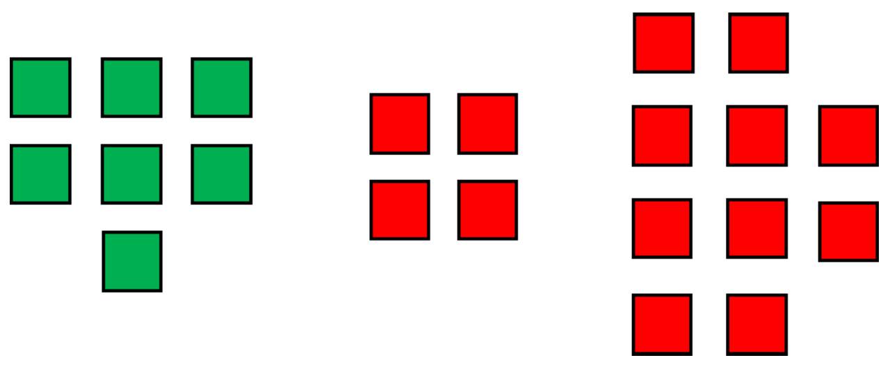
It is best done as an activity. Pick any three integers, say 7, ‒4 and ‒10 and represent them as piles of appropriate counters, i.e., 1st pile with 7 green counters, 2nd pile with 4 red counters, etc. (Figure 4). Now the sum 7 + (‒4) + (−10) will be all three piles combined into one. If only two piles can be combined at each step, then step 1 can be combining 1st and 2nd pile, i.e., the addition 7 + (−4) and step 2 can be combining the 3rd pile with this, i.e., adding −10 to the sum 7 + (−4) or [7 + (−4)] + (−10). On the other hand, step 1 can also be combining 2nd and 3rd pile or (−4) + (−10) with step 2 as combining 1st pile with this, i.e., adding 7 or 7 + [(−4) + (−10)]. Both lead to the combination of all three piles into one with no extra counter coming in or going out. So, the two sums must be equal, i.e., [7 + (−4)] + (−10) = 7 + [(−4) + (−10)]. The removal of zero pairs, i.e., pairs of green-red counters can happen after the three piles have been combined.

Observe that the three integers were chosen arbitrarily, and this can be extended (at least as a thought experiment) for any three integers regardless of how far they are from zero.

There are 14 possibilities:

1. All 3 positive
2. 2 positive and 1 negative

3. 1 positive and 2 negative

• Positive + negative + negative
• Negative + positive + negative
• Negative + negative + positive

4. All 3 negative

The above illustration is an example of 3a with sum < 0. We leave the rest for the reader to explore.

Defining multiplication for integers is tricky since no model does the job completely. There are three cases involving negative numbers and multiplication − (a) negative × positive, (b) positive × negative, and (c) negative × negative. The NCERT textbook does a good job for integers by extending multiplication tables. The Integer chapter of Class 7 textbook deals with the above three cases separately and without assuming commutativity. However, several other textbooks assume commutativity and treat (a) and (b) as equivalent. We attempt to first define or make sense of each of the above kind of products and then justify the properties.

Let us establish the following key facts case by case (\(m\) and \(n\) are any whole numbers):

• Negative × positive = negative
  This is done using the notion of repeated addition, i.e., (−4) × 3 = (−4) + (−4) + (−4) = −12. Now repeated addition can be modelled using the counters, which in this case would be negative ones. It can be argued that this is identical to the positive × positive case i.e., 4 × 3 except for the colour of the counters. Or in other words, it generates the same array of 4 × 3 counters except for the colour. So, this array has 4 × 3 negative counters and thus represents the integer −(4 × 3). Therefore, (−4) × 3 = −(4 × 3). Note that 4 and 3 can be replaced by any whole numbers and the same argument holds. So, we have established the general case (−\(m\)) × \(n\) = −(\(m\) × \(n\)) … (1)
• Positive × negative = negative
  This is explored by extending the multiplication table of \(m\) beyond \(n\) = 1 to \(n\) = 0 and then towards \(n\) < 0 maintaining the pattern observed in the table. As we move up the table of \(m\) from \(n\) = 4, 3, 2, etc., we notice that the product is reducing by \(m\) in each step. This way or otherwise, we get that \(m\) × 0 = 0. So, the next step would be \(m\) × (−1) = 0 − \(m\) = −\(m\). This approach can be combined with skip counting on the number line to realize that \(m\) × (−\(n\)) is \(n\) skips of \(m\) lengths each starting from zero towards left or the negative side. Now, this is the same as \(n\) times repeated addition of −\(m\), i.e., (−\(m\)) × \(n\). So, \(m\) × (−\(n\)) = (−\(m\)) × \(n\) and therefore \(m\) × (−\(n\)) = −(\(m\) × \(n\)) … (2). Note that this is not commutativity.
• Negative × negative = positive
  This combines the previous two cases. It starts with creating a table for (−\(m\)) and then extending to \(n\) < 0. In this case, as we move up from \(n\) = 3, 2, 1, etc., the product becomes −3\(m\), −2\(m\), −\(m\). So, the product increases by \(m\) in each step. So, (−\(m\)) × 0 = 0. Combining this with skip counting on the number line, (−\(m\)) × (−1) = 0 + \(m\) = \(m\). And in general (−\(m\)) × (−\(n\)) is \(n\) skips of \(m\) steps from zero towards right or the positive side which is the same as \(m\) × \(n\). Therefore, (−\(m\)) × (−\(n\)) = \(m\) × \(n\) … (3)

However, there is no such model to establish similar meaning for rational numbers − e.g. how should one define (−3/5) × (−7/4)? There is no real-life example suitable for children at an elementary level to make sense of such examples. Therefore, we want to fill this gap through the next article on a visual model of multiplication based on scaling with the use of number lines.

Coming to properties of multiplication, we would take a less hands-on approach since we have established some key results. This is also a gentle way of showing children how mathematical proofs are done, i.e., how established results can be used step by step to deduce something new.

Let us recap the three results:

For any two natural numbers \(n\) and \(m\)

1. \(m\) × (−\(n\)) = −(\(m\) × \(n\))
2. (−\(m\)) × \(n\) = −(\(m\) × \(n\))
3. (−\(m\)) × (−\(n\)) = \(m\) × \(n\)

Commutative Property of Multiplication

This can be done as an extension of the whole number approach with rectangular array using the above three results. However, the proofs are gentle enough for upper primary level and can help children get a flavour of how math builds up logically.

There are three possibilities similar to the ones for commutativity of addition.

We have already established

4. \(m\) × \(n\) = \(n\) × \(m\)

i.e., the positive × positive case which is identical to natural numbers in the Multiplication Handbook.

Now we want to show the remaining cases: positive-negative i.e. \(m\) × (−\(n\)) = (−\(n\)) × \(m\) and negative-negative i.e. (−\(m\)) × (−\(n\)) = (−\(n\)) × (−\(m\)) for any natural numbers \(m\) and \(n\).

Commutativity of cases involving zero are trivial.

Associative Property of Multiplication

As in associativity of addition, there are 8 possibilities:

1. \(m\) × \(n\) × \(p\)
2. \(m\) × \(n\) × (−\(p\))
3. \(m\) × (−\(n\)) × \(p\)
4. (−\(m\)) × \(n\) × \(p\)
5. \(m\) × (−\(n\)) × (−\(p\))
6. (−\(m\)) × \(n\) × (−\(p\))
7. (−\(m\)) × (−\(n\)) × \(p\)
8. (−\(m\)) × (−\(n\)) × (−\(p\))

Note that 1 is the whole number case which was established in the Multiplication Handbook, i.e., we have

5. (\(m\) × \(n\)) × \(p\) = \(m\) × (\(n\) × \(p\))

We have shown 3, 5 and 8 below and have left the rest for the reader to try.

2 and 4 can be shown in a similar way.

6 and 7 can be shown similarly.

Distributive Property of Multiplication

Unlike the above two, the distributive property involves both addition and multiplication. So, we could not come up with a proof, but the array worked out. Here (1)−(3) will be used to create the array or the product given the integers.

There are 8 possibilities:

1. Positive × the sum

• Positive × (positive + positive)
• Positive × (positive + negative)

1. Sum > 0
2. Sum < 0

• Positive × (negative + negative)

2. Negative × the sum

• Negative × (positive + positive)
• Negative × (positive + negative)

1. Sum > 0
2. Sum < 0

• Negative × (negative + negative)

Note that 1a is identical to the whole number case shown in Multiplication Handbook. Also, negative + positive = positive + negative by commutativity of addition which we have established already.

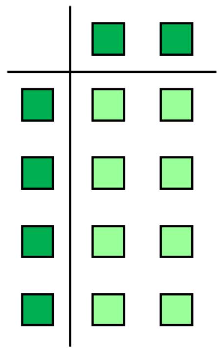
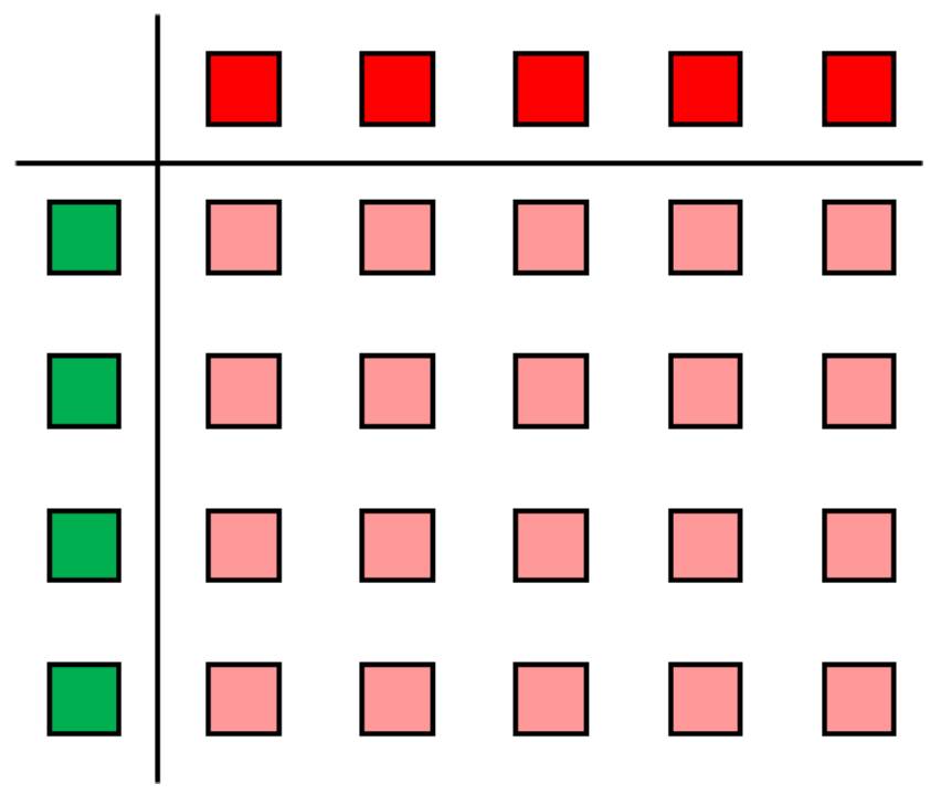
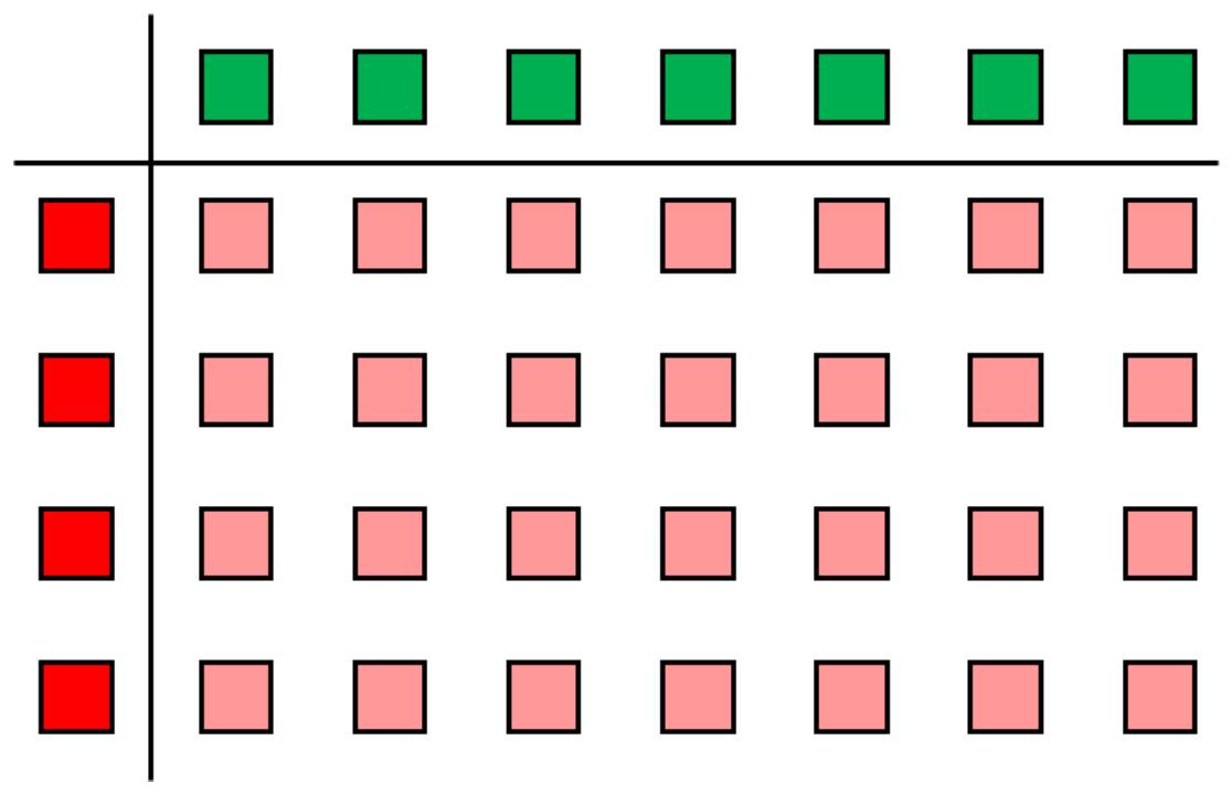
We have shown 1b(ii) and 2a. The reader is encouraged to try the rest.

The counters in the array, representing the product, are in a lighter shade to distinguish them from the counters in the borders, representing the factors.

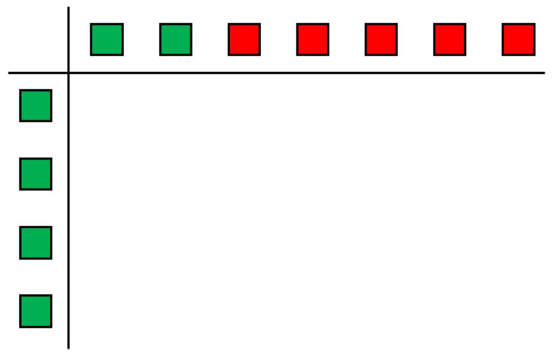
Step 1	4 × 2	4 × (-5)	4 × [2 + (-5)]
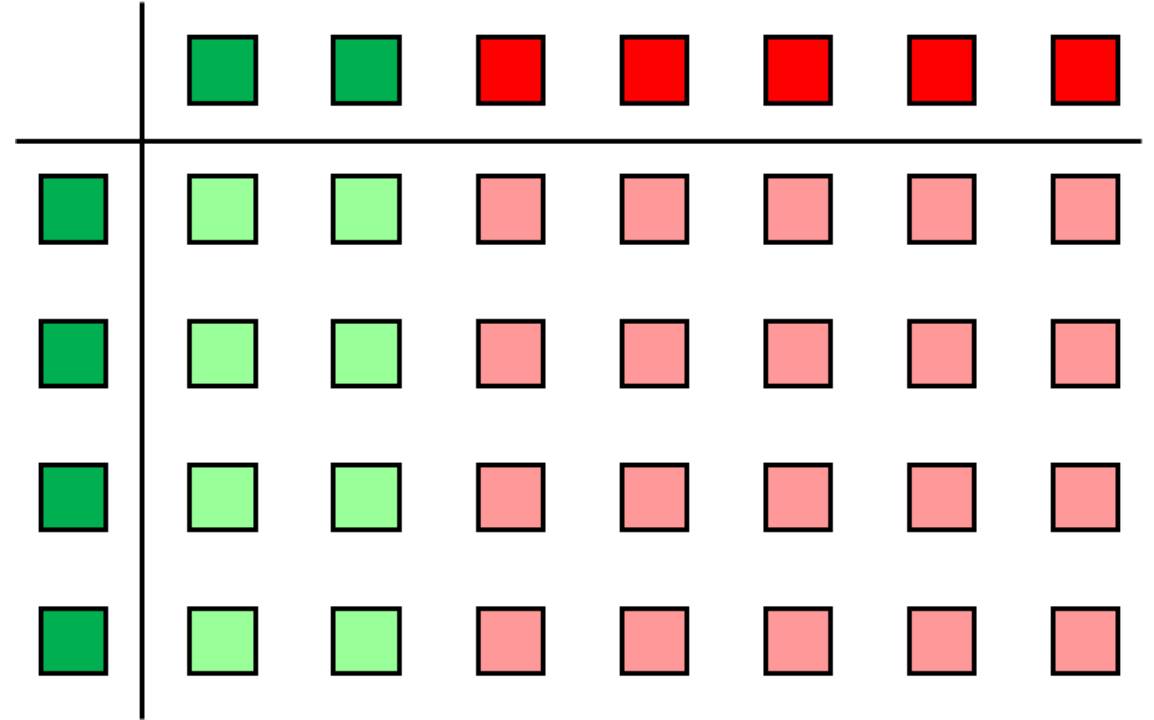
Step 2	4 × 2 + 4 × (-5)		Removing the zero pairs and filling in
Step 3	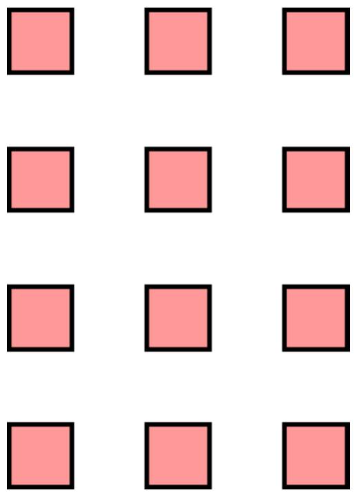Removing zero pairs and the borders		Removing the borders

(-4) × 2

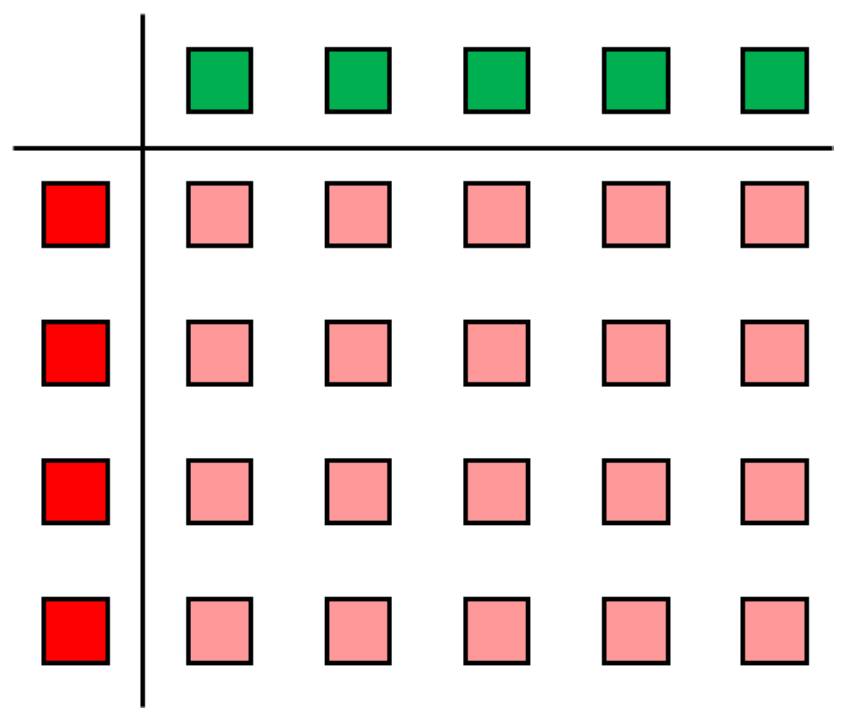
(-4) × 5

(-4) × [2 + 5]

Since the last arrays are identical for both, 4 × 2 + 4 × (−5) = 4 × [2 + (−5)]. Note the use of color for the array in 4 × (−5) based on (2).

In the following example of 2a, (1) is used to determine the colour of the arrays.

The 3rd picture of Figure 5 can be easily seen as the sum of the 1st and the 2nd i.e. (−4) × [2 + 5] = (−4) × 2 + (−4) × 5.

As in previous examples, observe that the integers chosen could have been arbitrarily distanced from zero. So, this procedure is valid for any three integers. In particular, if the 1st integer is zero then all the products are zero and the identity is trivially true. Similarly, if the 2nd or the 3rd integer is zero then one of the products become zero, i.e., one of the arrays vanishes and again the identity is trivially true.

The square colored counters arranged in a line can be generalized to coloured and therefore signed length and can be combined with the number line. If these counters are arranged in an array, they can be generalized to coloured, i.e., signed area. We did not face the need for signed volume. Also, this works for any 2-3 integers but not for rational or real numbers.

Rational and Real Numbers

Whole numbers were the easiest since they are discrete and non-negative and therefore can be modelled with counters. Fractions do not have the advantage of discreteness. But thanks to their non-negativity, they can be modelled by area (sometimes proportionate to length) and volume. Integers included negative numbers but could be modelled by coloured counters thanks to their discreteness. However, rational and real numbers are neither discrete, nor non-negative. So, they proved to be the most challenging sets. We will meet them in the next two articles.

¹The set of non-negative rational numbers include fractions and whole numbers. Henceforth, we will refer to this set as fractions.