Aryabhata and the Construction of the First Trigonometric Table

Introduction

We routinely use our calculator to obtain the sine of a given angle. (In earlier times we used published tables!) Little do we realize that a debt of gratitude is owed to the fifth century Indian savant Aryabhata who was the first to tell us about the sine function and create the first table of sines — in his seminal work, the Aryabhatiya (499 CE). In this article, we describe the trigonometric identities used by Aryabhata to obtain the table of sines.

The Indian mathematical tradition is largely word-based. Results are mentioned but derivations are omitted. The Aryabhatiya with more than 100 cryptic, super-compressed verses of dense mathematics is a prime example. In order to make our presentation pedagogical we take a unit circle and measure angles in degrees or radians instead of the (now) archaic notation in the Aryabhatiya and its commentators. We show that Aryabhata’s sine table entails taking the difference of the sine of two closely spaced angles and then taking the second sine difference. We also show that the trigonometric identities are the same as those in the finite difference calculus one uses nowadays to numerically obtain the first and second derivatives of the sine function. We follow this with a brief discussion. An understanding of these identities and preparation of the sine table will enable the reader to get an appreciation of the path-breaking work of Aryabhata. At the end, we suggest a few problems and invite the reader to try their hand at solving them.

The Aryabhatiya consists of 121 cryptic verses, dense and laden with meaning [1, 2]. The work is divided into 4 parts or padas: the Gitikapada (13 verses), Ganitapada (33 verses; the mathematics part), the Kalkriyapada (25 verses) and Golapada (50 verses; the astronomy part, which is better known than the others). There are two verses in Ganitapada describing the solution of the linear Diophantine equation. This has received due recognition. Our focus will be on the trigonometry part in Ganitapada which in our view has suffered neglect.

Virtually every major Indian mathematician has commented on the Aryabhatiya. Often it is in terms of a formal Bhashya (Commentary). Table I lists some of them. Notable among them is the voluminous work Maha Bhashya of the 15th century mathematician Nilakantha Somaiyaji (1444–1544 CE). He was part of the Kerala school which, beginning with Madhava (1350–1420 CE), founded the calculus of trigonometric functions.

Bhaskara I	629 CE	Sankrit	Valabhi, Gujarat
Suryadeva Yajvan	1191CE	Sankrit	Gangaikonda-Colapuram
Parameshvara	1400 CE	Sankrit	Allathiyur, Kerala
Nilakantha Somayaji	1500 CE	Sankrit	Trikandiyur, Kerala
Kondadarma	unknown	Telugu	Andhra
Abul Hasan Ahwazi	800 CE	Arabic	Ahwar, Iran

The Ardha-Jya or Sine Function

Aryabhata lays down — for the first time in the history of mathematics — a definition of the sine function. He poetically describes the sine function as the half bow-string or the Ardha-Jya, and relates the cosine functions to the arrow or saar (see Figure 1). This is not the only example of poetry making an appearance in his mathematics. To describe the fact — heretical and revolutionary for those times and for long afterwards — that the Earth is rotating and the Sun is stationary, Aryabhata evokes the tranquil metaphor of a boat floating down the river and the stationary river bank which seems to move backwards. Also being a poet, Aryabhata composed the Aryabhatiya in verse form with over 100 verses, respecting the norms of grammar and metre.

The sine function is the half-chord AP of the unit circle in Figure 1:

\(\mathbf{sin\ \theta = \frac{AP}{OA} = AP \hspace{24px} (OA = 1)}\)

The circle may be large or small; correspondingly, \(AP\) and \(OA\) may be large or small, but the \(LHS\) is a function of \(\theta\) and is not dependent on the scale of the figure. All metrical properties related to the circle can be derived using trigonometric functions and the Pythagorean theorem (also known as the ‘Baudhayana’ or ‘Diagonal’ theorem [4]). For example, the geometric properties of a triangle can be related to the arcs of the circumscribing circle using the sine and cosine functions. Or the diagonals of the inscribed quadrilateral can be related to its sides. (A recent proof of the Pythagorean theorem using the the law of sines suggests that all metrical properties of a circle can by obtained using trigonometry alone [5].) By emphasizing the role of the half-chord, Aryabhata endowed circle geometry with metrical properties. This alone should qualify him as the founder of trigonometry. But he did more.

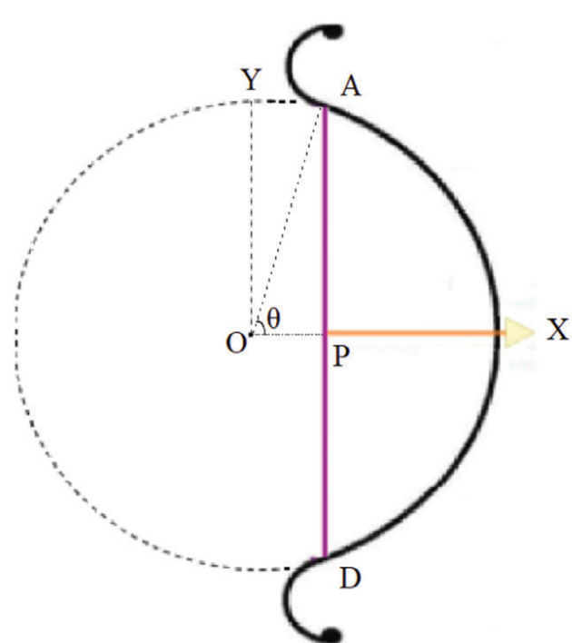
Note that the length of the half-chord \(AP\) is close to the length of the arc \(AX\) when the angle is small (i.e., \(sin\ \theta \approx \theta\) if \(\theta\) is small and in radians). This was known to Aryabhata. Similarly, \(sin\ 90^{o} = 1\), since then the half-chord is the same as the radius. In the 9th verse of Ganitapada he uses the property of an equilateral triangle and obtains \(sin\ 30^{o} = 1/2.\)

We pause to note that Aryabhata also states the value of \(\pi\) as 62832/20000 in the 10th verse. This value is 3.1416 and he is careful to state that this is ‘proximate’ (Asanna) suggesting that we can obtain better values for \(\pi\) with more effort. Here, the word Asanna or ‘proximate’ is to be distinguished from Sthula which is approximate or roughly equal.

The Difference Formula for Sine and Cosine

The 12th verse of Ganitapada plays a central role in the tabulation of the sine function. It is cryptic and to unravel its meaning we first need to obtain the difference formula for the sine. The presentation below relies on a number of sources: (i) The commentary of Nilakantha Somaiyaji [3]; (ii) the treatment of Shukla and Sarma [2]; (iii) and for the sake of ease of understanding we follow Divakaran [4] and work with a unit circle rather than one with radius \(3438^{1}\).

A convention adopted by earlier workers. Note that one radian is 3438 minutes; 2 π radians is 180◦; and 1◦ is 60 minutes.

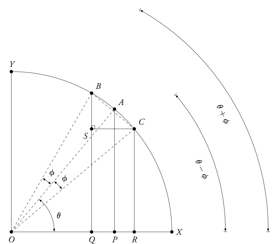
Figure 2 depicts a quadrant of the unit circle where \( OX = OY = 1.\) The arcs \(XA, XB\ and\ XC\) trace angles \(\theta , \theta + \phi\) and \(\theta – \phi\) respectively. The half-chords \(AP, BQ\) and \(CR\) are the corresponding sine functions. We drop a perpendicular CS from the circumference to the half-chord \(BQ\) as shown. According to his commentator Nilakantha Somaiyaji [3], Aryabhata obtained the relationship between the difference in the trigonometric functions by demonstrating that \(\triangle BSC\) and \(\triangle OPA\) are similar and exploiting this property in an ingenious manner. We trace his line of reasoning in the Appendix where we derive

\(sin(\theta + \phi) – sin(\theta – \phi) = 2 sin(\phi)\ cos \theta.\) (1)

The difference in the sines is thus proportional to the cosine of the mean angle.

\(cos(\theta + \phi) – cos(\theta – \phi) = -2 sin(\phi)\ cos \theta.\) (2)

The difference in the cosines is thus proportional to the (negative) of the sine of the mean angle.

Expressing the difference relations in another way, we get

\(sin(x) – sin(y) = 2sin \left(\frac{x-y}{2} \right) cos \left(\frac{x+y}{2} \right)\), and (3)

\(cos(x) – cos(y) = -2sin\left(\frac{x-y}{2} \right) sin\left(\frac{x+y}{2} \right) (4)\)

The Sine Table

Aryabhata begins with dividing the quadrant of the unit circle into 24 equal parts. He then obtains the values of the sines at fixed angles between 0 and \(\pi \text{/} 2 \) thus generating the sine table for \(\pi / 48 = 3.75^{o}\) , \(2\pi \text{/} 48 = 7.5^{\circ}\), \(3 \pi \text{/} 48 = 11.25^{\circ}\),… up to \(90^{\circ}\) (See Table 2). This table is given in verse 12 of the Gitikapada. It has been used by Indian astronomers (and astrologers!) in some form or another from 499 CE to the present. We shall see now how the table was generated.

As the quadrant is divided into 24 equal parts, let us take \(\varepsilon = \frac {\pi}{48}\) . Let us take \(\phi = \varepsilon/2\) where \(\varepsilon\) is small. We now compute the differences of successive values of sine and cosine for the increment of \(\varepsilon\). In other words, we compute the differences \(\delta s_{n}\) and \(\delta c_{n}\) defined below.

\(\delta s_{n} := sin\ n\varepsilon – sin(n-1)\varepsilon\), and

\(\delta c_{n} := cos\ n\varepsilon – cos(n-1)\varepsilon\)

where n varies from 0 to 24.
Using the equations (3) and (4), we get

\(\delta s_{n} = sin\ n\varepsilon – sin(n – 1)\varepsilon = 2\ sin\left (\frac{n\varepsilon – (n – 1)\varepsilon}{2} \right) cos \left (\frac{n\varepsilon + (n – 1)\varepsilon}{2} \right) = 2 sin \left( \frac{\varepsilon}{2}\right) cos \left(\left(n – \frac{1}{2} \right) \varepsilon \right) (5)\)

and

\(\delta c_{n} = cos\ n\varepsilon – cos(n – 1)\varepsilon = -2 sin\left (\frac{n\varepsilon – (n – 1)\varepsilon}{2} \right) sin \left (\frac{n\varepsilon + (n – 1)\varepsilon}{2} \right)= -2\ sin\left(\frac{\varepsilon}{2} \right) sin \left (\left( n-\frac{1}{2} \right)\varepsilon \right) (6)\)

We introduce the shorthand \(s_{\alpha}\) to write \(sin (\alpha \varepsilon)\) and \(c_{\alpha}\) to write \(cos (\alpha \varepsilon)\) and restate the equations (5) and (6) as

The above is a pair of coupled difference equations, and it was Aryabhata’s insight to take the second difference, namely

\(\delta^2 s_{n}=\delta s_{n} – \delta s_{n-1} = 2s_{\frac{1}{2}} \left(c_{\left( n-\frac{1}{2} \right)} – c_{\left(n-\frac{3}{2}\right)}\right) =-4s^{2}_{\frac{1}{2}} s_{n-1} \) (9) from equation(8)

Thus the second difference of the sines is proportional to the sine itself. The next step is to represent the \(RHS\) in terms of a recursion. We observe that \(s_{n} \) on the \(RHS\) of equation (9) may be written as

\(s_{n} = s_{n} + \left(s_{n-1} – s_{n-1} \right) + \left(s_{n-2} – s_{n-2} \right) + … + \left(s_{1} – s_{1} \right) + \left(s_{0} + s_{0} \right) \)

\(= \left(s_{n} – s_{n-1} \right) + \left(s_{n-1} – s_{n-2} \right) + … + \left(s_{1} – s_{0} \right) + s_{0} = \delta s_{n} + \delta s_{n-1} + … + \delta s_{1} + 0 \)

\(=\displaystyle\sum_{m=1}^{n} \delta s_{m}\)

Thus

Thus we get a recursion relation where the second difference of the sines is expressed in terms of all previously obtained first and second sine differences. To initiate the recursion, we need \(\delta s_{1}\) which is \(s_{1} – s_{0} = sin\ \varepsilon – sin\ 0 \approx \varepsilon\), since for small angles the half-chord and the corresponding arc are equal, as stated in the previous section.

Using the recursion relation we can generate Aryabhata’s celebrated sine table, taking \(\pi = 3.1416\) and \(sin\ \varepsilon = \varepsilon = 0.0654 (= 225^{‘} )\).

Table 2 depicts some typical values of the sine function as well as the value of the sine multiplied by 3438 (the so called ‘Rsine’ of Aryabhata). We see that this matches Aryabhata’s sine table to ±1 minute. For example, \(\theta = \pi/6\) gives 1719 minutes. For comparison, we also give the current accepted value of \(sin \theta\) to four decimal points. Note that Aryabhata takes angles only till \(\theta = \pi/2\); he seems aware of the fact that going further is unnecessary given the periodic nature of the sine function.

θ	sin θ (Aryabhata)	sin θ (minutes)	sin θ (modern)
π/48	0.0654	225	0.0654
2π/48	0.1305	449	0.1305
3π/48	0.1951	671	0.1951
4π/48	0.2588	890	0.2588
5π/48	0.3214	1105	0.3214
6π/48	0.3827	1315	0.3827
7π/48	0.4423	1520	0.4423
8π/48	0.5000	1719	0.5000
9π/48	0.5556	1910	0.5556
10π/48	0.6088	2093	0.6088
11π/48	0.6594	2267	0.6593
12π/48	0.7072	2431	0.7071
13π/48	0.7519	2585	0.7518
14π/48	0.7935	2728	0.7934
15π/48	0.8316	2859	0.8315
16π/48	0.8662	2978	0.8660
17π/48	0.8971	3084	0.8969
18π/48	0.9241	3177	0.9239
19π/48	0.9472	3256	0.9469
20π/48	0.9662	3322	0.9659
21π/48	0.9812	3373	0.9808
22π/48	0.9919	3410	0.9914
23π/48	0.9983	3432	0.9979
24π/48	1.0005	3439	1.0000

Finite Difference Calculus

Of greater relevance is the fact that the sine (or cosine) difference formulae foreshadow finite difference calculus, a popular numerical technique in this age of computation. Rewriting equations (1) and (2) with \(\phi = \varepsilon\),

Aryabhata took ε to be π/48. But he also stated that its value is yateshtani or ‘as per our wish’ (Verse 11, Ganitapada). Some took it to be π/96; others (like Brahmagupta) took it as π/12 or \(15^{o}\). If we take ε to be sufficiently small, we have our classic formula for finite difference calculus. Noting that \(2 sin\ \frac{\varepsilon}{2} \approx \varepsilon\) we have the finite difference version of the derivative of sine,

\(\frac{sin\ \theta}{d \theta} = cos\ \theta\),

and similarly for the cosine,

\(\frac{cos\ \theta}{d \theta} = -sin\ \theta\),

Let us illustrate this with an example. We know that \(sin\ 37^{o} \approx 0.6 \), and \(sin\ 30^{o} = 0.5\). The difference in angle is \(7^{o}\) which in radians is 0.122. Thus the derivative of sine of the mean angle \(33.5^{o}\) from equation (11) is

\(\delta\ sin\ \theta / \delta \theta = (0.6 – 0.5) / 0.122 = .82. \)

Looking up the sine table or the calculator yields \(cos\ 33.5^{o} = 0.83\). Similarly equations (9) yields the second derivatives namely

\(\delta^{2} sin\ \theta / \delta^{2} \theta \approx -sin\ \theta \)

\(\delta^{2} cos\ \theta / \delta^{2} \theta \approx -cos\ \theta\)

The above are now called central difference approximations to the first derivative and the second derivative. Naturally, Aryabhata does not use the term ‘finite difference calculus’ (or ‘calculus’). But similar methods are now used to numerically solve differential equations. The student will recognize the above as a standard solution of the classical simple harmonic oscillator. We note in passing that Newton’s II Law and the famous Schrödinger equation of quantum mechanics are both second-order differential equations.

Discussion

One can discern a continuity in Indian mathematics, however tenuous, from pre-Vedic times (prior to 1000 BCE) till the 1800s. A striking example is the influence of Aryabhatiya on major Indian mathematicians who followed him including Madhava (1350 CE) who founded Calculus [4]; as also the influence on Aryabhata of the mathematics which preceded him [6, 7].

To reiterate, Aryabhata seems aware that

1. \( sin\ 0^{o} = 0\);
2. The sine of a small angle is itself, as the small arc is ‘almost equal’ to the half-chord;
3. \( sin\ 30^{o} = 1/2\) (Ganitapada verse 9);
4. \( sin\ 90^{o} = 1\);
5. The sine function is periodic, so he prudently does not extend the computation to angles greater than \(90^{o}\).

Then, in a remarkably insightful way, he lays down the recursion relation for sine differences which enables one to generate the sine table. It is this work, more than his solution to the linear Diophantine equation (verses 31 and 32 of Ganitapada) which establishes him as a genius and one of the brightest stars in the firmament of world mathematics.

The sine table can also be generated using the half-angle formula. This was demonstrated in the Panchasiddhantika, a text written barely 50 years after the appearance of Aryabhatiya [8]. As pointed out, a feature of the Aryabhata’s difference relation is how modern it is. It can readily be seen to be essentially the same as finite difference calculus. It led to the development of the calculus of trigonometric functions by Madhava (1350 CE) and his disciples along the banks of the Nila river in Kerala. This school is variously called the Nila [4] and the Aryabhata school [7]. Another aspect to note is that Bhaskara II (1100 CE) used the division of the great circle into parts of magnitude 2π/96 to carry out discrete integration and obtain the (correct) expressions for the surface area and the volume of a sphere. Jyesthdeva of the Nila (or Aryabhata) school in his work Yuktibhasa derived the same results using calculus (circa 1500 CE). Aryabhata can thus legitimately be called the founder of trigonometry.

To sum up, the Aryabhatiya exercised a tremendous influence over Indian mathematicians for over a thousand years. For a book with just over one hundred pithy verses, its legacy remains unparalleled in the scientific world. We hope that our article will give our young audience an introduction to his work and will serve as an inspiration.

Acknowledgement

One of the authors (VAS) would like to place on record the many useful discussions he had with Prof. P. P. Divakaran.